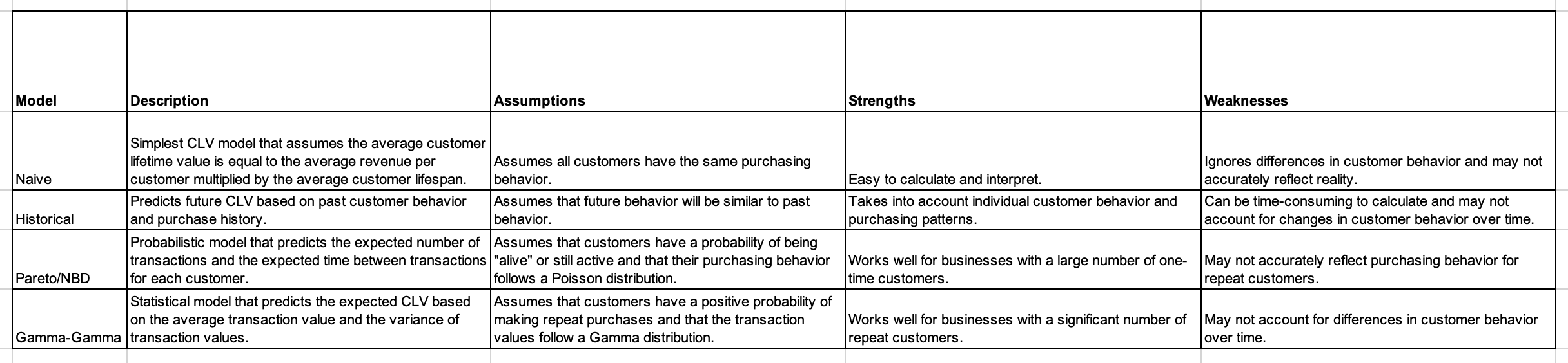
CLV Models

Knowing which customer is worth how much in their lifetimes

At its core, RFM segmentation is one of many techniques employed to predict and improve the Customer Lifetime Value (CLV).

Customer Lifetime Value (CLV) is a critical metric that helps retailers to understand the long-term value of a customer to the business. Retailers can use CLV to identify high-value customers, prioritize marketing efforts, and personalize the customer experience.

Given these different options, we would like to examine how we will code for these ones. The first and the second are pretty obvious. Let us examine the code for the rest of the two.

No matter which model which model you choose or you create a brand new model, the steps are sort of identicial:

1. Determine the time period for CLV calculation: Typically, the time period used for CLV calculation ranges from 12 to 24 months, depending on the nature of the business and the length of the customer lifecycle.

2. Split the data into training and testing sets: This is necessary to evaluate the performance of the model. The training set is used to train the model, while the testing set is used to evaluate the model's performance on unseen data.

3. Choose a CLV model: There are various models that can be used to calculate CLV, including the Pareto/NBD model, Gamma-Gamma model, and RFM (Recency, Frequency, Monetary) model. Each model has its own advantages and limitations, so it's important to choose the model that best fits your business needs.

4. Train the CLV model: This involves using the training data to fit the chosen model. The parameters of the model are adjusted to minimize the difference between the predicted and actual values of customer behavior, such as purchase frequency and monetary value.

5. Evaluate the performance of the CLV model: Use the testing set to evaluate the performance of the CLV model. You can use metrics such as mean squared error, mean absolute error, or R-squared to evaluate the model's accuracy.

6. Apply the CLV model: Once the model has been trained and validated, you can apply it to new customers to predict their future value to the business. This can inform marketing and customer acquisition strategies, as well as customer segmentation and retention efforts.

Here is some sample code for building a simple CLV model using the Pareto/NBD model:

import lifetimes

# create a summary dataframe for customer transaction data
summary_df = lifetimes.utils.summary_data_from_transaction_data(
    df_transactions, 
    customer_id_col='customer_id', 
    datetime_col='transaction_date', 
    monetary_value_col='order_total')

# fit the Pareto/NBD model
model = lifetimes.ParetoNBDFitter(penalizer_coef=0.0)
model.fit(summary_df['frequency'], summary_df['recency'], summary_df['T'])

# predict future customer transactions
summary_df['predicted_purchases'] = model.predict(
    summary_df['T'], 
    summary_df['frequency'], 
    summary_df['recency'], 
    summary_df['monetary_value'])

# calculate CLV
summary_df['clv'] = lifetimes.customer_lifetime_value(
    model, 
    summary_df['frequency'], 
    summary_df['recency'], 
    summary_df['T'], 
    summary_df['monetary_value'], 
    time=12, 
    discount_rate=0.01)

This code uses the lifetimes library in Python, which provides tools for fitting and evaluating CLV models. In this example, we use the Pareto/NBD model to predict future customer transactions and calculate CLV over a 12-month time period. The code outputs a summary dataframe with predicted purchases and CLV for each customer, which can be used to inform marketing and retention strategies

Here's some sample Python code for implementing the Gamma-Gamma model in the lifetimes package:

import pandas as pd
from lifetimes import GammaGammaFitter

# Load data with monetary value and frequency columns
df = pd.read_csv('customer_data.csv')

# Fit the Gamma-Gamma model to the data
ggf = GammaGammaFitter()
ggf.fit(df['frequency'], df['monetary_value'])

# Calculate the expected average CLV for each customer
df['expected_clv'] = ggf.customer_lifetime_value(
    transaction_prediction_model=None,
    monetary_value=df['monetary_value'],
    frequency=df['frequency'],
    time=12, # Time period in months for which to calculate CLV
    discount_rate=0.01 # Annual discount rate for future cash flows
)

# Display the results
print(df[['customer_id', 'monetary_value', 'frequency', 'expected_clv']])

In this example, we first load the customer data into a Pandas DataFrame that includes columns for the customer's monetary value (i.e., the average value of each transaction) and frequency (i.e., the number of transactions made by the customer). We then fit the Gamma-Gamma model to the data using the GammaGammaFitter class from the lifetimes package.

Once the model is fit, we can use the customer_lifetime_value() method to calculate the expected average CLV for each customer over a specified time period (in this case, 12 months) and at a given discount rate (in this case, 1%). Finally, we add the calculated CLV values to the original DataFrame and print out the results.

Note that in this example, we've assumed that the transaction prediction model is None, which means that we're only using the Gamma-Gamma model to predict the monetary value of each customer's future transactions, not the timing or frequency of those transactions. If desired, we could also use a separate model (such as the BG/NBD model) to predict the customer's future transaction frequency, and then combine the predictions from both models to generate a more accurate CLV estimate.